Sunday, February 19, 2017

Exercise 3: Cartographic Fundamentals

3D Sandbox Terrain
Figure 1. Sandbox Terrain that includes an areal image measured in centimeters, four 3D side views of the terrain, and a reference map.

The location of the sandbox was on the University’s campus to the East of Phillips Hall, across the road of Roosevelt Ave. About 100 ft. from the loading dock of Phillips, the sandbox was placed next to a shed. In Figure 1, the map is broken down into 4 angles of the terrain from ArcScene and a large image of an areal view of the sandbox. Specifically looking at the areal view, the goal of the terrain was to include a ridge, hill, depression, valley, and a plain. The terrain was measured in centimeters. The hill is the highest elevated area on the map if you look at the white color. The statistics show that the maximum value is 21.74 cm (Table 1). The minimum value is 6.86 cm, which can be identifies in the dark green areas along the red ridge in Figure 1. The mean elevation of this terrain was calculated as 12.47 cm. This is approximately the same elevation as the plain, located in the lower right corner of the image. The four side view images are shown from each corner of the terrain. The dimensions of the sandbox are expressed as 114 x 114 cm. Each view is labeled as to what direction it is viewing from: NW, NE, SE, SW. The X and Y-axis are also labeled to be identified as it changes when the corner view rotates.

Table 1. Elevation (cm) statistics of the Sandbox Terrain calculated in ArcMap. 

Hadleyville Cemetery 
The data for the Hadleyville Cemetery Gravestones was collected on September 14, 2016 using a phantom drone at 50 meters in altitude. The raster image was projected in WGS 1984. This site is located in Hadleyville in Eau Claire County, WI.
Figure 2. Hadleyville Cemetery with the last names on the gravestones labeled.
Many of the gravestones in Figure 2 are grouped by families. Many of these plots of land placed next to one another by plots of land that families typically purchase together. The top ri ght corner consists of many Session's and McDonald's and Jacot's below them. The bottom right corner does not have many gravestones yet. This could be for future deaths, there is however, four stones in the lower part. The upper left corner of the grave does not have many head stones, but the left side in general contains the names like Hadley or Cleasby.
Figure 3. Hadleyville Cemetery with the year the gravestones were placed labeled on it.
Figure 3 shows the Year of Death (YOD) of each grave. Splitting the graves into three sections, the left side contains many graves from the late 1800s. A few of the graves are in the early 1900s, but this could be due to having family plots of land pre-purchased for other members of the family. This pattern continues for the middle of the graveyard as well. But the left side has changes the year of death. The graves are mainly in the 1900s, earlier and later. There is also one grade that defines the year of death in 2006.
Figure 4. Hadleyville Cemetery with the the Year of Death (YOD) represented with a graduated symbol for the newer stones being larger and the older stones having a smaller symbol. 
Another figure symbolically demonstrates the age of the stones (Figure 4). The stones range from 1859 to 2006. They are split into five classes. The smaller symbols represent older stones, while the larger symbols are younger stones. The larger symbols are mainly grouped together in upper right corner and the upper middle. However, there are still larger symbols scattered around the grave. Many of the smaller symbols are located in the midde of the graveyard and to the left. There are also many more smaller symbols than bigger ones.
Figure 5. Hadleyville Cemetery showing which gravestones are still standing or not.
The final map is shows if the grave stones are still standing or not. Looking at the layout in Figure 5, there is only 5 red dots. Therefore out of all the gravestones in the Hadleyville Cemetery, there is only 5 that are no longer standing.

Sunday, February 12, 2017

Exercise 2: Sandbox Survey

Part 1: Introduction

  • Discuss what you did in the previous lab.
    • In the previous lab, an elevation surface of a terrain was constructed in a square meter sandbox. The profile had to include a ridge, hill, depression, valley, and a plain. Finally, the group will be able to map out the elevated surface using original survey technique.
    • For the lab, our group chose to create a grid that allowed for 20 points on the X-axis and 20 points on the Y-axis. The grid consisted of 400 squares, where we measured a point in the top-right corner to achieve our 400 data samples.
  • Discuss what the term 'Data Normalization' means, and how that relates to this lab
    • Data normalization is the process of organizing data into tables in such a way that the results can be used in a database to create points that can then be used to be manipulated further. 
    • The data points of x, y, z were normalized into three columns in an excel data sheet. The points were then projected into ArcMap into a grid that presented the grid that was created on the sandbox. By doing this, then a 3D model can be created of the profile by using ArcScene. 
  • Discuss your data points, and how the interpolation procedure in today’s lab will help to visualize that data. 
    • After perfecting the data to create the grid that turned out really well, the next processes was to interpolate. This will allow for a 3D model of our Sandbox Terrain to be implemented. By using different interpolation methods, we will then decide which best presents the sand profile. 


Part 2: Methods
You were shown how to bring your data into 3D scene. You were also shown how to export that scene for use in a map layout.
    • After the data was normalized into 3 columns of X, Y, and Z, the XY data was added into ArcMap. A grid was created of the X and Y values, which is shown in Figure 1. 
Figure 1. The origional grid, before any interpolations. 
    • From there, we experimented with a few different interpolation methods such as IDW, Kriging, Natural Neighbors, Spline and TIN.
    • "In most GIS literature, areal interpolation specifically means the reaggregation of data from one set of polygons (the source polygons) to another set of polygons (the target polygons). Predictions and standard errors can be made for all points within and between the input polygons, and predictions (along with standard errors) can then be reaggregated back to a new set of polygons." (ESRI 2016)
      • "IDW (inverse distance weighted) interpolation determines cell values using a linearly weighted combination of a set of sample points." (ESRI 2016)
      • "Kriging is based on statistical models that include autocorrelation. Kriging assumes that the distance or direction between sample points reflects a spatial correlation that can be used to explain variation in the surface." (ESRI 2016)
      • "Natural Neighbor interpolation tool finds the closest subset of input samples to a query point and applies weights to them based on proportionate areas to interpolate a value" (ESRI 2016).
      • "Spline uses an interpolation method that estimates values using a mathematical function that minimizes overall surface curvature, resulting in a smooth surface that passes exactly through the input points." (ESRI 2016)
      • "TIN (triangular irregular networks) have been used by the GIS community for many years and are a digital means to represent surface morphology. TINs are a form of vector-based digital geographic data and are constructed by triangulating a set of vertices (points). The vertices are connected with a series of edges to form a network of triangles." (ESRI 2016)
  • In what format did you export your 3D scene image?
    • From ArcScene, I exported my 3D image as a JPEG, so that it would be easier to show the clarity and availability of the data model. 
  • What orientation did you decide upon?
    • For the orientation, I chose a tilted side view of the 3D scene image that is viewed from a corner and shows elevation as well as some of the areal view of the image. 
  • How did you decide to reflect scale? Why does one need to place scale and orientation in these exports?
    • The measurements of the grid was 114 x 114 cm. On the model, I drew in a line that showed how each side was 114 cm. 


Part 3: Results/Discussion 1

  • Discuss the results of each method in detail, and refer to the figure, noting where there are issues with the output.
  • Revisit your previous lab and make sure you do a detailed job of combining what you did previously with this lab to have what you did carefully documented.
  • Discuss with your group what you could do differently in a follow up survey
For the IDW method, every 6 cm our group measured an elevation point (z). In Figure , you can see there there is a small hill or bump that was created where each point was taken and a slight depression where there was an absence in data. The Hill and Valley that our group created were not well mapped to scale with this method. 


 Figure 2. IDW Interpolation Method

When the Kriging Interpolation was used, the profile was smoothed out more than the IDW. However, Figure 3 demonstrates that there is still areas where a few points were exemplified or depressions were formed because of no measurements being taken in that specific spot. 
Figure 3. Kriging Interpolation Method 

The Natural Neighbors Interpolation provided an output that had some inconsistencies in it as well. The 3D image created unaccurate depressions and hills that surround the data points like the Kriging and IDW interpolation. In Figure 4, there almost seems to be a square shape to the layout of the landscape. 
 Figure 4. Natural Neighbors Interpolation Method

Figure 5 demonstrates an interpolation method that provides a smooth and representative sample landscape of the sandbox. The Spline method smooths out the areas that lack the measurements and connects them to the adjacent points. In this figure, the hill, valley, plain, ridge, and depression are easily seen. 
Figure 5. Spline Interpolation Method

The last interpolation method that was looked at was the TIN. The TIN does no use a smoothing technique or show an accurate idea of what the landscape of the sandbox was supposed to look like (Figure 6). TIN uses a series of triangles that connect other interpolation points together from the defined measured points from the data. The series of triangles then make up a sample of the landscape. 
Figure 6. TIN Method

Part 4: Revisit your survey (optional)
Evaluate your best interpolation method and assess where you have data that is lacking.

  • If your survey was bad, remake up your terrain to the best of your ability to match your previous terrain.
  • Now redo your survey, taking note of where your survey previously lacked detail.
  • Perform an interpolation using only the ONE best interpolation method you decided upon
  • Discuss the results of this 'redo', and relate the quality of the output to your previous survey.
After 5 methods were gone through, the lab was revisited with the interpolation method that I thought was the most representative of my sandbox terrain. Using the Spline with Barriers Interpolation Method, I redid my terrain with the grid points added as an overlay layer to the 3D scene imagery (Figure 7). I also added an areal image to compare the the overlay of the points with the image that is tilted towards its side. Not much of the terrain did change after I redid it. North of the Hill, there was supposed to be a depression that I attempted to adjust the measurements, but it still did not show. I assume this is either due to an error in the measurements or the tool smooths out the area so much that the depression begins to not be as prominent. 


Figure 7. Spline with Barriers Interpolation Method with the Grid of Points

Part 5: Summary/Conclusions

  • How does this survey relate to other field based surveys? How is the concept the same? How is it different?
    • These surveys can be used a reference point to demonstrate topography of the area of study. There will also be times where measuring a particular terrain could have impacts on knowing what the slope is, for example, a hill or depression. Knowing the slope can have an impact on providing evidence for how acknowledge a particular land use for a given area. 
  • Is it always realistic to perform such a detailed grid based survey?
    • No, depending on the size of the study area or study site it would be impractical to have that many data points due to time or too large of an area. 
  • Can interpolation methods be used for data other than elevation? How so? Provide examples?
    • Interpolation methods could also be used for any other data that contains intervals, such as weather maps or temperature maps. This could establish boundaries of areas that are projected to receive more snow or rain, or collectively show what areas experience the highest or lowest temperatures at any given length of time. 

References
ESRI. 2016. How IDW Works. Accessed February 12, 2017.      http://desktop.arcgis.com/en/arcmap/latest/tools/3d-analyst-toolbox/how-idw-works.htm.
ESRI. 2016. What is a TIN surface? Accessed February 12, 2017.  http://desktop.arcgis.com/en/arcmap/latest/manage-data/tin/fundamentals-of-tin-surfaces.htm.


Monday, February 6, 2017

Exercise 1: Creation of a Digital Elevation Surface

Introduction

·         Define what sampling means, with a strong focus/emphasis on what it means to sample in a spatial perspective.
o   Sample can be defined as part or single item that is representative of a larger group. Spatially a sampling method needs to be able to allow for enough data to create a stronger representation of the area or object that is being sampled. 
·         List out the various sampling techniques
o   Simple Random Sampling (SRS)
o   Stratified Sampling
o   Cluster Sampling
o   Systematic Sampling
o   Multistage Sampling (in which some of the methods above are combined in stages)
o   Multiphase Sampling
o   Convenience Sample
o   Purposive Sample
·         What is the lab objective(s)
o   The objective of this lab is to use geospatial thinking to construct an elevation surface of a terrain that is located in a square meter sandbox. The profile had to include a ridge, hill, depression, valley, and a plain (Figure 1). Finally, the group will be able to map out the elevated surface using original survey technique.

Figure 1. Photo of an top view of what the profile our group created with all the requirements.

Methods

·         What is the sampling technique you chose to use? Why? What other methods is this similar to and why did you not use them?
o   We used systematic sampling so we could create a method that allows for the most data points that will target the majority of the grid.
·         List out the location of your sample plot. Be as specific as possible going from general to specific.
o   The sandbox was located on the University’s campus.
o   It was to the East of Phillips Hall, across the road of Roosevelt Ave.
o   About 100 ft. from the loading dock of Phillips to the sandbox located next to a shed.
·         What are the materials you are using?
o   Materials that were used were a meter stick, string and tacks, a flag, and a square meter sandbox.
·         How did you set up your sampling scheme? Spacing?
o   For this lab, our group chose to create a grid that allowed for 20 points on the X-axis and 20 points on the Y-axis as shown in Figure 2.
o   The grid consisted of 400 squares, where we measured a point in the top-right corner to achieve our 400 data samples.

Figure 2. Grid of our profile with x and y-axis defined. 

·         How did you address your zero elevation (sea level)?
o   We measured the height of the sandbox to get a defined sea level of 15 cm.
·         How was the data entered/recorded? Why did you choose this data entry method?
o   We created a 3 column table with X-Y-Z as the headers for each column. The x-axis and the y-axis was defined in the row, before the elevation of Z was recorded. The group then took the difference between the string and where the sand ends in order to figure out the elevation or Z (Figure 3).
o   With only a notebook as a form of recording data, creating columns was the most efficient way of entering data before it was entered on a spreadsheet into a table.

Figure 3. Meter stick measuring at one of our sample points by measuring the space between the sand and the string. 

Results/Discussion

·         What was the resulting number of sample points you recorded?
o   400 sample points
·         Discuss the sample values? What was the minimum value, the maximum, the mean, standard deviation, etc.
o   
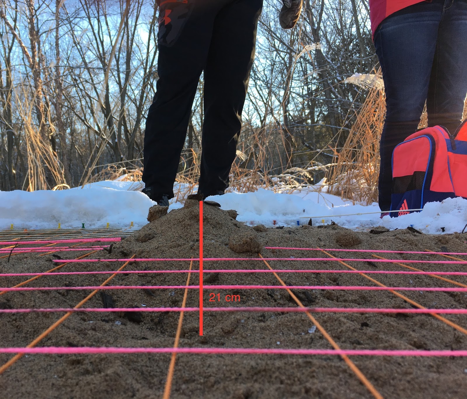
The range of the sample points was 14, with the minimum value being 7 cm and the maximum value being 21 cm (Figure 4).
o   The mean was 12.48 cm, with a standard deviation of 2.14 cm.
o   The mode was 12.
o   Our sea level was also established at 15 cm.
Figure 4. Photo of our hill and maximum Z-value. 
·         Did the sampling relate to the method you chose, or could have another method met your objective better?
o   For this particular activity, we could not have used any of the random samples. Therefore, systematic was the best choice.
·         Did your sampling technique change over the survey, or did your group stick to the original plan? How does this relate to your resulting data set?

o   The sample that we chose was the one that we stuck with throughout our data collection.
·         What problems were encountered during the sampling, and how were those problems overcome.
o   During the sampling, often times the spot that we were going to sample next was often lost. But we were able to follow along with the grid system of our data collection in the notes.
o   There were often times that the meter stick was to big more measuring elevation and some of the data points may not be as accurate as they should.

Conclusion

·         How does your sampling relate to the definition of sampling and the sampling methods out there?
o   While often times, there needs to be a random sample in order for much of the data collection to be considered unbiased and representative of the larger sample. In this case in order to gather enough data to accurately represent the elevations of different points in our sandbox, the sampling method needed to be systematic.
·         Why use sampling in spatial situation?
o   Sampling eliminates the bias and persuasion of how one would collect the data.
·         How does this activity relate to sampling spatial data over larger areas?
o   By using this small scale model of the sandbox, we could conduct another sample of a larger area with the same grid technique as well as use the sampling method we chose for this exercise for a larger area as well.
·         Using the numbers, you gathered, did your survey perform an adequate job of sampling the area you were tasked to sample? How might you refine your survey to accommodate the sampling density desired.

o   It is already noticeable in that sample shows variation in the landscape based on the higher numbers in some areas, lower in other, and a consistency of numbers in the depression. To refine the measuring aspect of the survey, I would find a more efficient and accurate use of measuring. The metering stick may not have been the best way to get accurate measurements of the elevation.